Anomaly Detection for Time Series Data: Part 2

In our previous post, Anomaly Detection for Time Series Data: Part 1, we looked into the importance of anomaly detection and the impact that it can have on business. We also discussed the different types of anomalies, introduced algorithms useful for their detection, and described some use cases.

In this second part of the series, we’re going to further explore a few algorithms that are useful for detecting anomalies, including:

• ARIMA
• STL
• Twitter Seasonal Hybrid ESD
• Isolation Forest
• Elliptic Envelope
• Quartile Based Outlier

To start with, let’s first look at the algorithm which is most commonly used for forecasting related problems and which can also be used as an anomaly detection technique.

ARIMA (AutoRegressive Integrated Moving Average)

Let’s understand how this model works using sales at an ice cream shop as an example.

The shop owner wants to estimate sales for the current month, based on repeat customers from previous months. For this, he looks at the sales of the last few months and checks how these figures have changed over time, and he then restocks the ice cream inventory accordingly. 

So for future strategies, the shopkeeper can make use of the above techniques — AR, MA, and Differencing — to have an intelligent analysis of the factors affecting his sales and restock the inventory accordingly.

ARIMA is based on the assumption that previous values carry inherent information and can be used to predict future values.

The model “learns” from the behaviour of the data and tries to forecast the values. If forecasted values are significantly different from actual values, then it is an anomaly.

A standard notation used for the above model ->  ARIMA ( AR->p, I->d, MA->q )

Where parameters p, d, q represents:-

• p: lag order – Number of lag observations included in the model
  
• d: degree of differencing – The number of times the observations are differenced (subtract the previous value from the current value, required to make the time series stationary*).
  
• q: order of moving average – The size of the moving average window

*Stationary Time Series -> Series whose statistical properties such as mean, variance, etc. remain constant over time.

Extra – Detailed insights on ( p , d , q ) with code implementation Source1 , Source2 , Source3

Example of the time series with an anomaly

Despite being simple in terms of approach, there are some limitations that can’t be ignored:

• The ARIMA model is specifically built for time series (sequential) data, but real-world data doesn’t always carry information from previous data, which could result in less accurate predictions.
• It can only capture linear dependencies with the past.
• Another limitation stems from the subjectivity involved in determining the (p,d,q) order of the model.

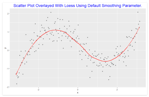
STL (Seasonal and Trend Decomposition Using Loess)

This is a method used for time series decomposition into trend, seasonality, and remainder components, using Loess smoothing (a smooth line passing through a scatter plot to help discover clear patterns, and relationships between variables).

Source

Let’s see How STL can be used with the example–

Suppose a person is tracking e-commerce sales revenue and looking for overall trends in this revenue over time. He knows that, in general, consumers buy more products in the 4th quarter as compared to others due to various reasons such as festivals, weddings, etc. So if he wants to analyze the pattern without considering this seasonality and check if revenue is rising in general, then he can use STL to decompose the time series and analyze the trend component separately.

Source

In time series decomposition, the Seasonal component is calculated first and removed in order to calculate the Trend component. The Remainder is simply calculated by removing the above two components from the original series.

Time Series =  Seasonality + Trend + Remainder

• Seasonality – When some pattern is repeating itself after a fixed periodicity. 
  For example: festive seasons like Christmas/New Year occur at a fixed period gap of one year — periodicity is 1 in this case

• Trend – Whether data is increasing/decreasing or remaining constant as time passes. 
  For example: stock market trends, which either go up or down depending on external factors

• Remainder – Everything that is left over

Individual components are explained in-depth in Blog: Part1

From an anomaly-detection perspective, the basic idea is that if you have a time series with a regular pattern (seasonality + trend), you can isolate it using the STL algorithm. Everything left over is called the remainder which we need to monitor for anomalies.

Example – 

Time Series Data – 

Isolate Trend and Seasonality ( Periodicity ) from the above time series – 

Remainder –  we need to monitor it for anomaly detection.

Anomalies  – Highlighted Red Points

STL is a versatile and robust method for decomposing time series. The only drawback is that it does not detect multiple seasonal components from the series and only considers the one with the highest frequency. 

For series with multiple seasonalities, a slight variation of the STL algorithm known as MSTL (Multiple Seasonal-Trend decomposition using LOESS) can be considered. 

The above discussed technique (STL) is also used by one of the advanced algorithms for anomaly detection SHESD which is a bit more complex with relation to the above two but has more applicability on real-life datasets.

S-H-ESD (Seasonal Hybrid ESD)

S-H-ESD is an algorithm developed by Twitter, built upon a Generalized ESD (Extreme Studentized Deviate) Test for detecting anomalies. 

The steps taken in S-H-ESD implementation:

1. Decompose the time series into STL decomposition (trend, seasonality, remainder).
2. Then, calculate the Median Absolute Deviation (MAD) if hybrid (otherwise the median).
   In the presence of anomalies, the remainder component can get corrupted. So to prevent this MEAN was replaced by MAD while performing the ESD Test.
   
   MAD (Median absolute deviation) – Subtract the median from each value in the data set and make the difference positive. Add up these quantities and divide by the number of values in the data set.

3. Perform a Generalized ESD test on the remainder, which we calculate as: `R = ts – seasonality – MAD or median.

Twitter’s SHESD package has multiple other functionalities such as detecting the direction of anomalies, window of interest, piecewise approximation for long time series, and has visual support as well.

Advantages of using this algorithm: 

• It can be used for low sample datasets to detect anomalies. 
• It is able to detect both local and global anomalies even in the presence of trend and seasonality.

Source

The drawback of using the MAD approach is that the execution time of the algorithm increases as median/MAD requires sorted data. Therefore, in cases where the time series under consideration is large but with a relatively low anomaly count, it is advisable to use S-ESD.

Isolation Forest

As its name suggests, this algorithm is built on an approach similar to decision trees with the concept that as we go deeper into the tree, the chances of detecting anomalies will decrease as compared to the shorter branches.

The main reason for the above is that the tree is able to split and separate the point from other observations way easier in shorter branches.

Example: 

Suppose a company has 10,000+ employees. We can consider as many variables as we want to: age, salary, birthplace, job title, etc.

Now if we talk about the Founder of the company, he might surely be an outlier compared to the other employees. 

We fit a tree on the above data and define each terminal leaf as being an employee of the company.

So Isolation Forest should filter out the Founder within fewer branches as compared to a new employee in the company.

As we can see from the above diagram, the Founder was separated out by the first split itself as surely, from the given employee dataset, he is an outlier.

Trees in isolation forests will be formed by randomly selected features from randomly sampled data and will be split by random threshold values until all points are isolated.

Decision Tree is a supervised learning algorithm and the Isolation Forest is an unsupervised learning algorithm. (Read: Supervised and Unsupervised Learning Algorithm)

Source

After model training is completed, the results will be the aggregate of the score obtained for each point when it is traversed through each binary tree separately, and the score will be given based on how deep an individual point has to traverse in a tree to get separated.

Anomaly score = 1  For General Points

Anomaly score = -1  For Anomaly

In (a) Highlighted point(Red) can be separated by three partitions, so it can be considered as an anomaly by the algorithm.
Reason – Easily separated with less number of partitions, shorter branch.

In (b) Highlighted point(Red) is separated after nine partitions, so the algorithm will not classify it as an anomaly in this case.
Reason – More number of partitions, more depth

This algorithm has a significant advantage over other methods as it does not use the similarity, distance, or density measurements of the dataset, which are usually computationally expensive. 

Isolation Forest (original paper) complexity grows linearly as it uses the sub-sampling technique. 

Thus, it can be applied to large datasets with many irrelevant variables, for both supervised as well as unsupervised use cases. 

The limitation of the above algorithm is that it will not work and/or not provide good results, either for:

• the contextual anomaly detection use cases 
• the anomalies present in multivariate time series data.

Elliptic Envelope

Suppose we have some data that represents *Normal distribution. And we try to fit most of the points by deciding on some shape that will help us to identify observations. The one which does not go along with the most data can be considered an outlier.

Elliptic Envelope is one such algorithm that works on the above concept where we define an elliptical shape to engage most of the data. **Covariance is estimated for the points inside the shape, which is further used to calculate ***Mahalanobis distance and get the outliers.

* Normal Distribution (also known as Gaussian distribution) – Bell-Shaped probability distribution curve that is symmetric about the mean. It shows that data near the mean occur more frequently as compared to data at the edges of the curve.

** Covariance refers to the measure of how two variables in a data set are related to each other.
(If we take the scaled form of covariance then it will be called correlation.)

*** Mahalanobis Distance – Distance metric that finds the distance between a point and a distribution.

Source

For Normal distributed data, the distance of observation to the mode of the distribution (value that appears most often in a set of data values) can be computed using its Mahalanobis distance. This calculation is very sensitive to the outlier points.

 -1 is allotted for anomalies

 +1 for normal data or in-liers.

Extra:  In-Depth Implementation with code

The concept behind the Elliptic Envelope is very simple, and it works well if the data follows Normal distribution. But it also has a few known limitations such as:

• It does not work well on non-normal distributed data.
• Implementation of this model is a bit tricky as we need to define the proportion of outliers in the dataset— a value we don’t know.
• Outlier detection from covariance estimation may break or not perform well in high-dimensional settings.

Now let us look at a basic statistical approach that is commonly used to remove anomalies while solving most machine learning problems.

Quartile-Based Outlier

If you have data with outliers and you need to get to the middle of the data. The mean is not the right choice as it is affected by the presence of outliers, so we should go with the median instead. 

Now, to define the outliers we define the range in this algorithm, and if points lie outside that range then it is considered an anomaly.

Range is defined as:

Lower Limit = Q1-1.5*IQR,   Upper Limit = Q3 + 1.5*IQR,   IQR = Q3 – Q1

IQR – Inter Quartile Range – Used to measure variability and is generally calculated by the difference between Q3 and Q1

The dataset is sorted in ascending order and divided into four parts. Values used to divide these are called quartiles. Q1, Q2, and Q3 represent the 25th, 50th, and 75th percentile of the data respectively.

Mostly we use the box-plot method for the above case representation.

Source

IQR is one of the most popular and simple statistical approaches to identify anomalies in the data. In this, we don’t need to check on the assumption of normality, and we don’t need to know the proportion of outliers in advance. 

A few limitations of this algorithm: 

• It doesn’t work if seasonal patterns are present in the dataset.
• This technique is applied to individual features only, not for the whole set of features as in the Elliptic envelope.

Conclusion

Many algorithms can be used to detect anomalies in a dataset. We’ve discussed a few of them in this blog, but there are still many more that can be explored, such as Prophet, Luminol, ExactStorm, KNNCAD, Hotelling Approach, and DBSCAN.

Based on the type of data and industry, each algorithm has a different implementation and is used to detect different types of anomalies (Point, Collective, and Contextual Anomaly) in a dataset.

So, to be a good practitioner, knowing the assumptions behind each algorithms/methods and understanding their strengths and weaknesses is a must. This will help you decide when to use which method and under what circumstances.

For any use case, you should always start with the most basic approach and only then move to more complex models. Try to combine multiple techniques together to detect outliers as there is no single best technique. This will help to improve the overall result.

* * *